TCA in SVARs
Section 5.1 of Wegner et al. (2025) splits the effects of monetary policy into contemporaneous and non-contemporanous effects, the latter of which are linked to forward guidance and other non-conventional policies. In this example, we do the same. Before we begin, download both the code and the replication data. Make sure to put the data and the code into the same folder.
To ensure a clean environment, we recommend starting a new Matlab session. Alternatively, run the following lines to clear the workspace and console:
clear;
clc;
Next, add the TCA Toolbox to the Matlab path. You will likely have to adjust the file paths in the quotation marks:
addpath("~/Documents/repos/tca-matlab-toolbox/");
addpath("~/Documents/repos/tca-matlab-toolbox/plotting");
addpath("~/Documents/repos/tca-matlab-toolbox/models");
Finally, before coming to the analysis, load the replication data into a table:
data = readtable("./data.csv");Wegner et al. (2025) do the analysis for two internal instruments of monetary policy shocks: (1) the Gertler and Karadi (2015) instrument and (2) the Romer and Romer (2004) instrument. We split our analysis accordingly and start investigating the contemporanous and non-contemporaneous effects of monetary policy estimated using the Gertler and Karadi instrument.
Gertler Karadi
Gertler and Karadi (2015) derive an instrument for monetary policy shocks by extracting the surprise component of FOMC meetings from the change in Fed Funds Futures in a tight time window around these FOMC meetings. This instrument is contained in the data and named mp1_tc. Also contained in the data is the Romer and Romer (2004) instrument (rr_3) which we do not currently need.
To focus on the GK instrument, we filter the data for only the GK instrument, interest rates, output gap, commodity prices and inflation
keepCols = {'mp1_tc', 'ffr', 'ygap', 'infl', 'lpcom'};
dataGK = data(:, keepCols);
With the data at hand, our transmission channel analysis follows the common six steps.
1. Defining the model
The first step to any transmission channel analysis is to define the model. Here, we will go with a VAR model. We include the instrument in the VAR, thus effectively deciding that we identify the shock via an internal instrument.
model = VAR(dataGK, 4, 'trendExponents', 0:1);
model.fit();
2. Obtaining IRFs
Next, we obtain the total effects – the structural IRFs – by using the GK series as as internal instrument. We thus define our InternalInstrument identification method:
method = InternalInstrument('ffr');Structural IRFs can then be obtained by using IRF and providing the identificationMethod.
irfObj = model.IRF(40, 'identificationMethod', method);
irfs = irfObj.getIrfArray();
Although not strictly necessary, we normalise the shock’s size to 25bps. This can be achieved by mutiplying the structural IRFs, currently normalised to a 1pp increase, by 0.25.
irfs = irfs(:, 1, :) * 0.25;3. Defining the transmission matrix
The third step to any transmission channel analysis is the definition of the transmission matrix. Wegner et al. (2025) order the Fed Funds rate first, followed by all other variables. The implementation of internal instruments is slightly different here, requiring us to order the internal instrument first, followed by the Fed Funds rate, and all other variables. The transmission matrix can then be defined in the following way:
transmissionOrder = {'mp1_tc', 'ffr', 'ygap', 'infl', 'lpcom'};4. Defining transmission channels
The fourth step is to define the transmission channels. Wegner et al. (2025) focus on two channels that perfectly decompose the effect. They define the contemporanous channel of monetary policy as the effect of monetary policy going through a contemporanous adjustment in the federal funds rate. They then define the non-contemporaneous channel of monetary policy as the effect of monetary policy not going through a contemporanous adjustment in the federal funds rate – the complement of the contemporaneous channel. Note that according the Section 4.3 of Wegner et al. (2025) the effects through these channels are invariant to any re-ordering of inflation, commodity prices, and the output gap, as long as they are ordered after the Fed Funds rate.
The non-contemporanous channel can be defined in the following way:
channelNonContemp = model.notThrough('ffr', 0, transmissionOrder);The contemporanous channel can be defined in a similar way:
channelContemp = model.through('ffr', 0', transmissionOrder);5. Computing transmission effects
Transmission effects can now be computed using transmission. We must provide our InternalInstrument identificationMethod:
effectsNonContemp = model.transmission(1, channelNonContemp, transmissionOrder, 40, 'identificationMethod', method);
effectsContemp = model.transmission(1, channelContemp, transmissionOrder, 40, 'identificationMethod', method);
% adjusting for shock size
effectsNonContemp = effectsNonContemp * 0.25;
effectsContemp = effectsContemp * 0.25;
To double check whether everything worked, we check whether the two channels perfectly decompose the total effect. Very minor differences might exist due to numerical rounding.
max(vec(irfs - effectsContemp - effectsNonContemp))6. Visualising decomposition
Lastly, we visualise the decomposition using plotDecomposition. We must first define the channel names:
channelNames = ["Contemporaneous", "Non-Contemporaneous"];
cellChannelEffects = {effectsContemp, effectsNonContemp};
The decomposition for the effects of a monetary policy shock on the federal funds rate (the second variable in the data) can then be obtained in the following way:
fig = plotDecomposition(2, irfs, cellChannelEffects, channelNames);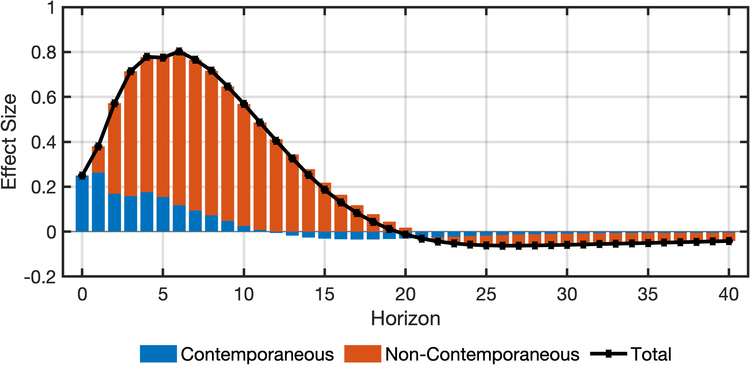
Similarly, the decomposition for the effects of a monetary policy shock on inflation (the fourth variable in the data) can be obtained in the following way:
fig = plotDecomposition(4, irfs, cellChannelEffects, channelNames);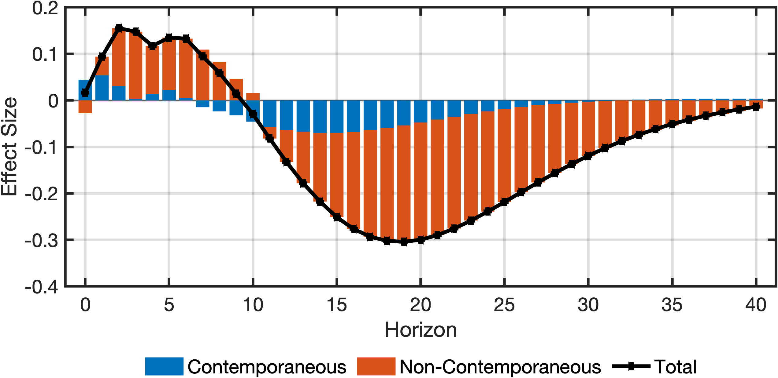
Romer and Romer
Most of the transmission channel analysis for the Romer and Romer (2004) instrument follows the same steps as for the Gertler and Karadi (2015) instrument. Below we highlight only the differences. For steps 2, 4, 5, 6, the same code as above can be used.
Before we start, we must first adjust the data and replace the GK with the RR instrument:
keepCols = {'rr_3', 'ffr', 'ygap', 'infl', 'lpcom'};
dataRR = data(:, keepCols);
1. Defining the model
Because the data has changed, our model definition changes slightly – the dataset name changes.
model = VAR(dataRR, 4, 'trendExponents', 0:1);
model.fit();
3. Defining transmission matrix
The transmission matrix remains largely the same, but the name of the instrument changes.
transmissionOrder = {'rr_3', 'ffr', 'ygap', 'infl', 'lpcom'};6. Visualising effects
While the code ramains the same, the graphs change.
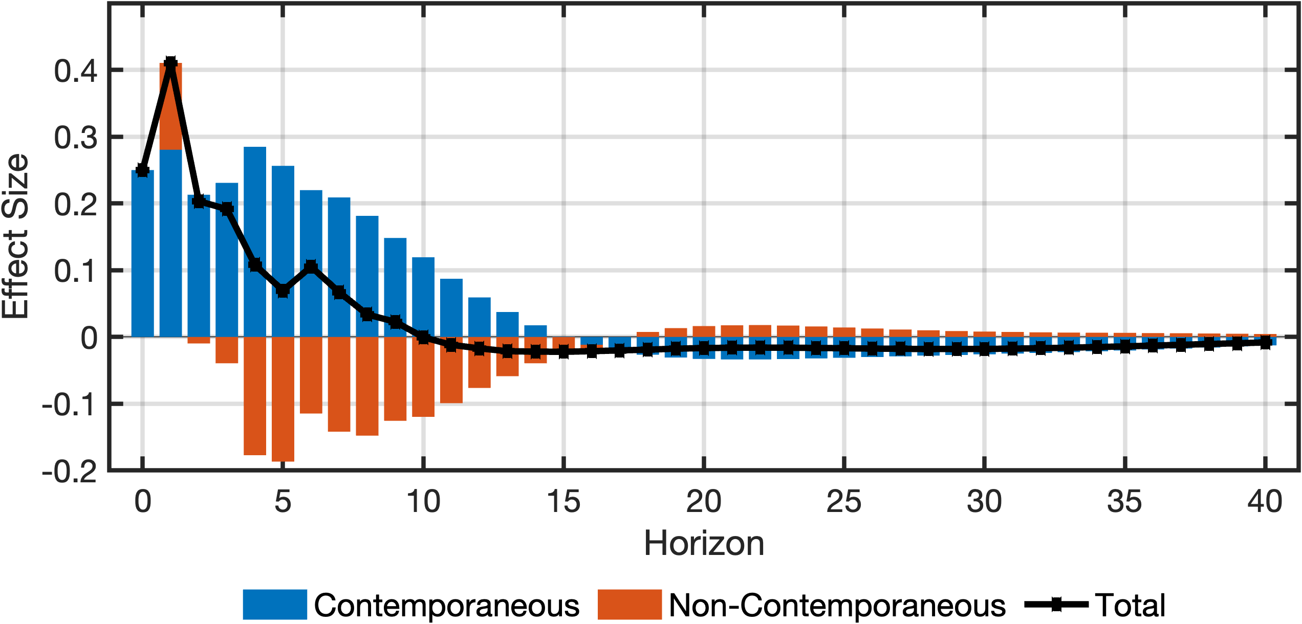
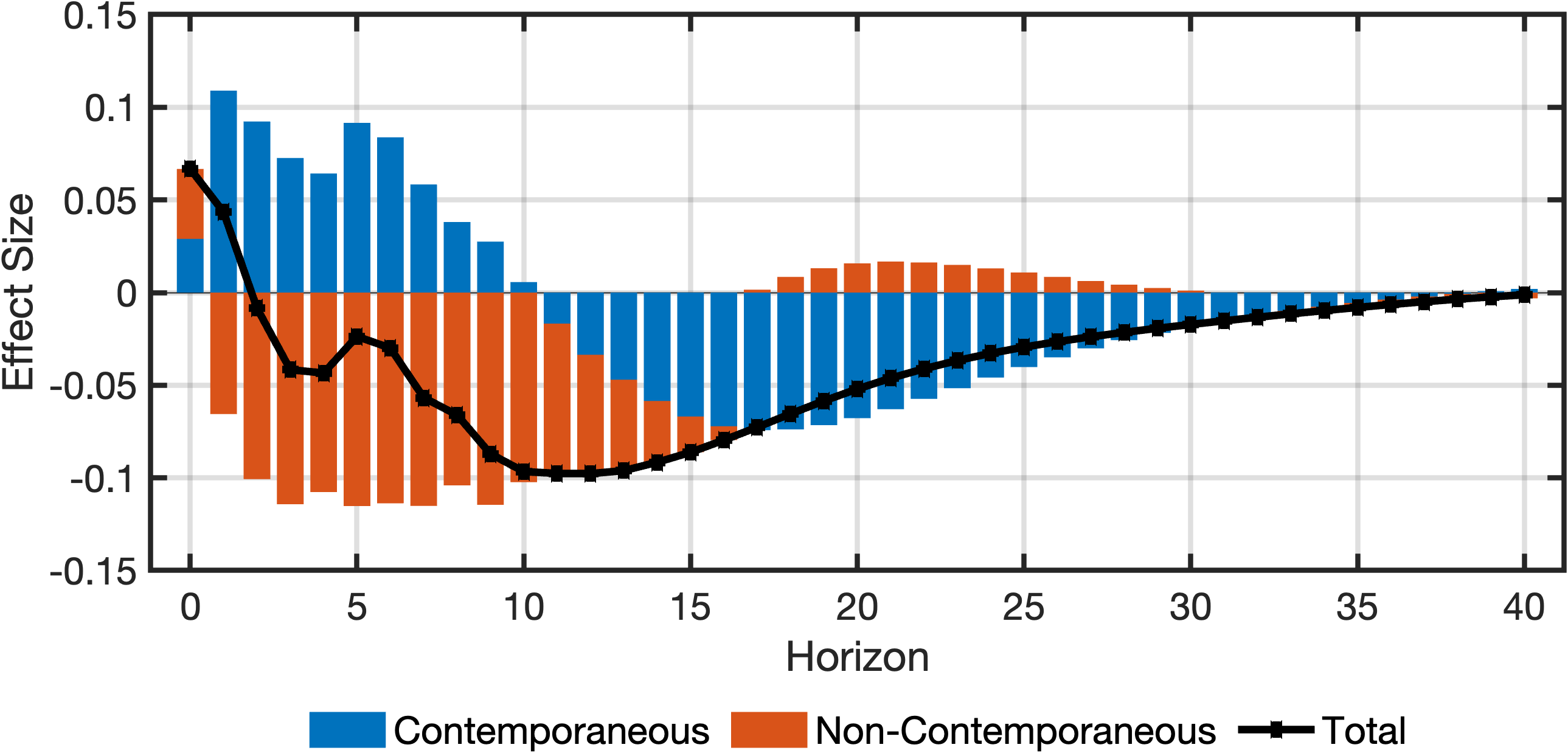
Minor differences between the decompositions here and the ones in the paper are due to how we obtain the Cholesky-orthogonalised IRFs. In the paper we estimate orthogonal IRFs using a VAR excluding the internal instrument. Here we include the internal instrument.