TCA in Local Projections

In this example, we examine the anticipation and implementation effects of government defense spending, closely following Section 5.2 in Wegner et al. (2025). Before beginning, download both the code and the replication data. Ensure that the data and code are placed in the same folder.

To ensure a clean environment, we recommend starting a new Julia session.

Next, add add the required packages to the environment. The following steps can be skipped if the packages already exist in the enrivonment.

] add TransmissionChannelAnalysis, DataFrames, CSV, CairoMakie, Makie

After adding the packages to the environment, load them:

using TransmissionChannelAnalysis
using DataFrames, CSV
using CairoMakie  # for plotting

Finally, before proceeding with the analysis, load the replication data into a table:

data = DataFrame(CSV.File("./data.csv"))

The remainder of this example follows the standard six-step approach.

1. Defining the model

We estimate structural impulse response functions (IRFs) using local projections (LPs). An LP model can be created using LP, specifying the treatment variable and maximum horizon. Wegner et al. (2025) use the defense spending series from Ramey (2016) as a direct measure of the shock. Thus, the treatment is newsy, and the maximum horizon is set to 20 periods.

model = LP(data, :newsy, 4, 0:20; include_constant=true)

The local projection can then be estimated using fit!:

fit!(model)

2. Obtaining total effects

Since newsy is treated as a direct measure of the shock, the effects of a government defense spending shock can be identified recursively by ordering the newsy series first. This recursive identification scheme can be defined using Recursive:

method = Recursive()

Using this Recursive identification scheme, structural IRFs can be obtained via IRF:

irfs = IRF(model, method, 20)
irfs = irfs.irfs[:, 1:1, :]

3. Defning the transmission matrix / order

The transmission matrix is defined as a vector of Symbol. Wegner et al. (2025) split the total effects into anticipation and implementation effects. They define the anticipation channel as effects that do not pass through actual government defense spending. Thus, it is logical to order gdef (government defense spending) as early as possible in the transmission matrix, but it must not precede the shock variable, newsy. The chosen transmission matrix is:

transmission_order = [:newsy, :gdef, :g, :y]

4. Defining the transmission channels

Wegner et al. (2025) define the anticipation channel as the effects of the government defense spending shock that do not pass through government defense spending at any period. This channel can be defined using not_through as follows:

anticipation_channel = not_through(model, :gdef, 0:20, transmission_order)

The implementation channel, representing effects passing through government defense spending in at least one period, is then the complement of the anticipation channel:

implementation_channel = !anticipation_channel

5. Computing transmission effects

Transmission effects are computed using transmission for the first 20 periods, considering the first shock, corresponding to the defense spending shock. Structural IRFs required for the computations are derived using the Recursive identification method defined earlier.

anticipation_effects = transmission(model, method, 1, anticipation_channel, transmission_order, 20)
implementation_effects = transmission(model, method, 1, implementation_channel, transmission_order, 20)

6. Visualising transmission effects

To visualise transmission effects, first define channel names and collect the effects in a vector:

teffects = [anticipation_effects, implementation_effects]
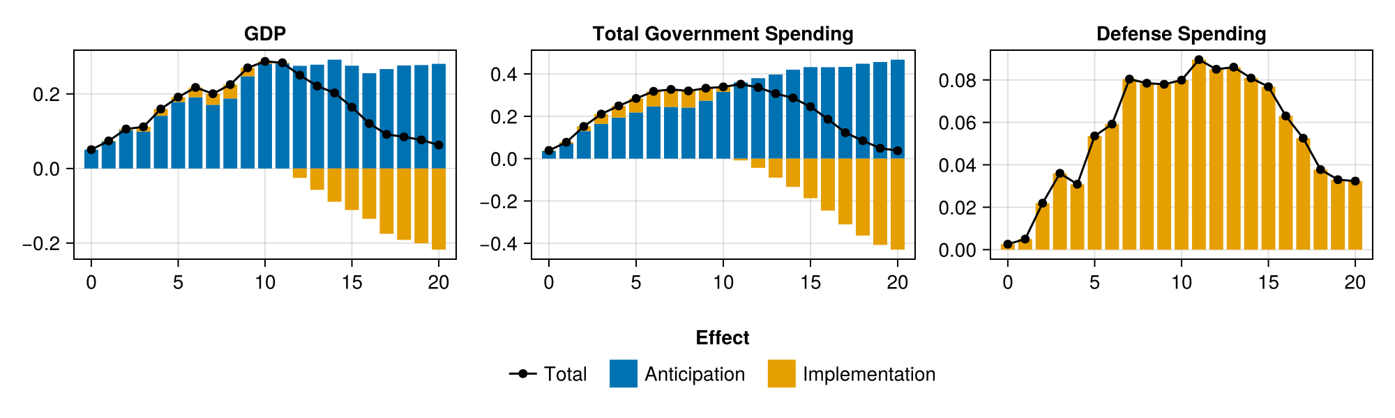
channel_names = ["Anticipation", "Implementation"]

The effects can then either be visualised one after another by using plot_decomposition or all together by creating a composite figure as below. To create the composite figure showing the decompositions for GDP, total government spending, and defense spending, we first create a new figure:

We then create a new axis at position [1, 1] into which we plot the decomposition of the defense spending shock on GDP using plot_decomposition!.

Similarly, we can plot the decomposition for total government spending and defense spending into positions [1, 2] and [1, 3], respectively.

Lastly, we can add a legend below the three plots using add_decomposition_legend!.

The figure below displays the decompositions.

Decomposition of a government defense spending shock into anticipation and implementation effects

References

Ramey, Valerie A. 2016. “Defense News Shocks, 1889 - 2015: Estimates Based on News Sources.” Manuscript. Univ. California San Diego. https://econweb.ucsd.edu/~vramey/research/Defense_News_Narrative.pdf.

Wegner, Enrico, Lenard Lieb, Stephan Smeekes, and Ines Wilms. 2025. “Transmission Channel Analysis in Dynamic Models.” 2025. https://doi.org/10.48550/arxiv.2405.18987.