TCA in DSGEs using Dynare
In this example, we replicate the results from Section 5.3 of Wegner et al. (2025). Before we begin, download both the code and the Dynare model. Make sure to unzip the Dynare model, and place both the sw2007.m script and the SW2007 folder into the same directory.
To ensure a clean environment, we recommend starting a new Matlab session. Alternatively, run the following lines to clear the workspace and console:
clear;
clc;
Computing the Linearised DSGE using Dynare
Section 5.3 of Wegner et al. (2025) studies the wage channel of a contractionary monetary policy shock using the DSGE model of Smets and Wouters (2007). To analyse this channel, we first obtain the model’s first-order approximation using Dynare.
To use Dynare and the TCA Toolbox, we first add both to the Matlab path. You will likely need to adjust the file paths in the quotation marks:
addpath("~/Documents/repos/tca-matlab-toolbox/")
addpath("~/Documents/repos/tca-matlab-toolbox/models/")
addpath("~/Documents/repos/tca-matlab-toolbox/plotting/")
addpath("/Applications/Dynare/6.3-arm64/matlab/")
Assuming the SW2007 folder is in the current directory, we can now generate the first-order approximation:
cd SW2007;
dynare SW2007;
cd ..;
clc;
TCA Setup
With the TCA Toolbox added to the path, we can create a DSGE model from Dynare’s output structures:
model = DSGE(M_, options_, oo_);TCA requires impulse response functions (IRFs) to decompose effects. We obtain them as follows, extracting the IRF array from the IRFContainer:
maxHorizon = 20;
irfObj = model.IRF(maxHorizon);
irfs = irfObj.getIrfArray();
Defining Transmission Channels
At this stage, we have the DSGE’s first-order solution and the IRFs. We can now define the transmission channels of interest.
First, define the transmission matrix. Following Wegner et al. (2025), we order variables so that interest rates (robs) come first, wages (dw) second, and inflation (pinfobs) last. The ordering of variables between wages and inflation does not matter1:
order = {'robs', 'dw', 'labobs', 'dc', 'dinve', 'dy', 'pinfobs'};Next, we define the transmission channels. The demand channel is defined as the effect that does not pass through wages (dw) during any period from 0 to 20. We define this channel using the notThrough function:
channelDemand = model.notThrough('dw', 0:maxHorizon, order);The wage channel, capturing any effect through wages in at least one period, is the complement:
channelWage = ~channelDemand;Computing Transmission Effects
We can now compute the transmission effects using the transmission method of the DSGE model. We specify the shock (em), the transmission channel, the transmission matrix, and the maximum horizon:
effectDemand = model.transmission('em', channelDemand, order, maxHorizon);
effectWage = model.transmission('em', channelWage, order, maxHorizon);
The output has the same structure as the original IRFs, with variables appearing in their original order and adjustments made for the defined shock size.
Visualising Transmission Effects
To better understand the transmission effects, we plot their decomposition. We first name the channels:
channelNames = ["Demand Channel", "Wage Channel"];Next, identify the indices of the outcome variable (inflation) and the shock (monetary policy shock em):
idxInflation = model.getVariableIdx('pinfobs');
idxShock = model.getShockIdx('em');
Then collect the transmission effects into a cell array:
cellChannelEffects = {effectDemand, effectWage};Finally, create the decomposition plot:
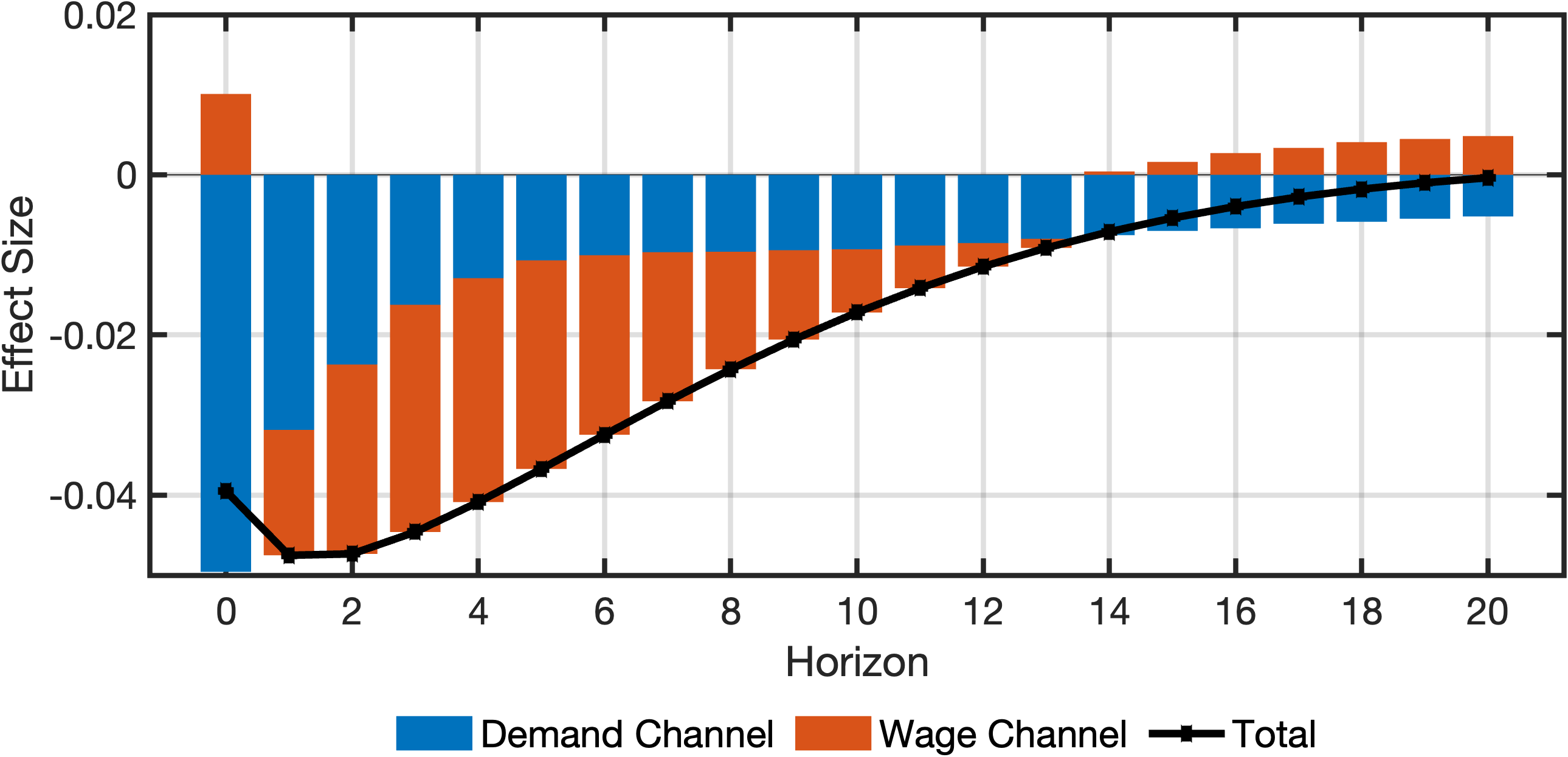
fig = plotDecomposition(idxInflation, irfs(:, idxShock, :), cellChannelEffects, channelNames);The plot shows:
- Total effect (black scatter-line)
- Effect through the demand channel (blue bars)
- Effect through the wage channel (red bars)
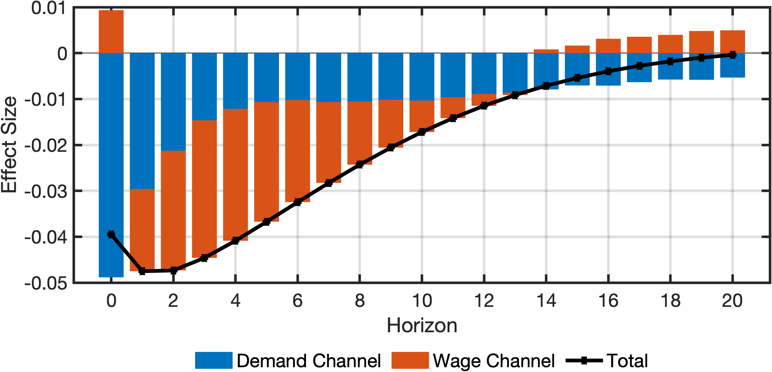
Using an Alternative Transmission Matrix
Wegner et al. (2025) also explore an alternative ordering, where wages are placed second to last. We define the new ordering as:
order = {'robs', 'labobs', 'dc', 'dinve', 'dy', 'dw', 'pinfobs'};Transmission channels and effects are then redefined and recomputed:
% Defining the channel again.
channelDemandAlt = model.notThrough('dw', 0:maxHorizon, order);
channelWageAlt = ~channelDemandAlt;
% Computing the alternative effects
effectDemandAlt = model.transmission('em', channelDemandAlt, order, maxHorizon);
effectWageAlt = model.transmission('em', channelWageAlt, order, maxHorizon);
The decomposition plot for the alternative ordering can be created as follows:
channelNames = ["Demand Channel", "Wage Channel"];
idxInflation = model.getVariableIdx("pinfobs");
idxShock = model.getShockIdx('em');
cellChannelEffectsAlt = {effectDemandAlt, effectWageAlt};
fig = plotDecomposition(idxInflation, irfs(:, idxShock, :), cellChannelEffectsAlt, channelNames);
The resulting plot mirrors the previous setup, with the only difference being the transmission matrix. The black scatter-line and the blue and red bars retain the same meaning as in the previous plot: the black scatter-line shows the total effect, the blue bars represent the demand channel, and the red bars represent the wage channel.
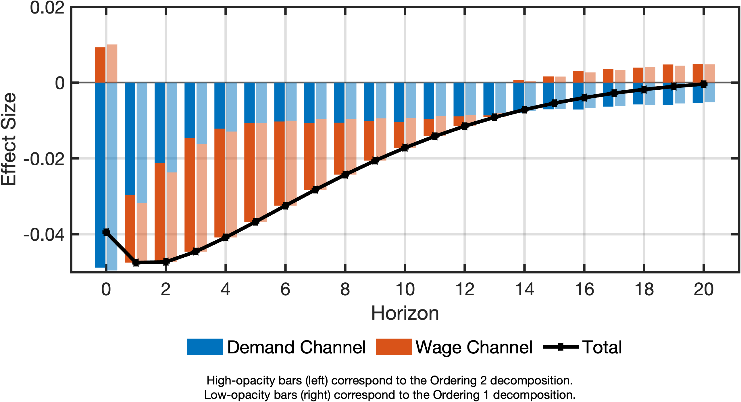
Comparing Transmission Effects of Different Transmission Matrices
We can place Figure 1 and Figure 2 side-by-side for comparison. As shown in Figure 3, differences are minor:
A more precise comparison uses the plotCompareDecompositions function. The following code generates Figure Figure 4:
fig = plotCompareDecompositions(...
    idxInflation, ...
    irfs(:, idxShock, :), ...
    cellChannelEffectsAlt, ...
    cellChannelEffects, ...
    channelNames, ...
    ["Ordering 2", "Ordering 1"] ...
);
Figure Figure 4 shows small but detectable differences, as predicted by theory.