TCA in Local Projections
In this example, we examine the anticipation and implementation effects of government defense spending, closely following Section 5.2 in Wegner et al. (2025). Before beginning, download both the code and the replication data. Ensure that the data and code are placed in the same folder.
For a clean working environment, we recommend starting a new Matlab session. Alternatively, clear the workspace and console by running:
clear;
clc;
Next, add the TCA Toolbox to the Matlab path. Adjust the file paths within the quotation marks as necessary:
addpath("~/Documents/repos/tca-matlab-toolbox/");
addpath("~/Documents/repos/tca-matlab-toolbox/plotting");
addpath("~/Documents/repos/tca-matlab-toolbox/models");
Finally, before proceeding with the analysis, load the replication data into a table:
data = readtable("./data.csv");The remainder of this example follows the standard six-step approach.
1. Defining the model
We estimate structural impulse response functions (IRFs) using local projections (LPs). An LP model can be created using LP, specifying the treatment variable and maximum horizon. Wegner et al. (2025) use the defense spending series from Ramey (2016) as a direct measure of the shock. Thus, the treatment is newsy, and the maximum horizon is set to 20 periods.
model = LP(data, 'newsy', 4, 0:20, 'includeConstant', true);The local projection can then be estimated using fit:
model.fit();2. Obtaining total effects
Since newsy is treated as a direct measure of the shock, the effects of a government defense spending shock can be identified recursively by ordering the newsy series first. This recursive identification scheme can be defined using Recursive:
method = Recursive()Using this Recursive identification scheme, structural IRFs can be obtained via IRF:
irfObj = model.IRF(20, 'identificationMethod', method);
irfs = irfObj.getIrfArray();
3. Defning the transmission matrix / order
The transmission matrix is defined as a cell array of char. Wegner et al. (2025) split the total effects into anticipation and implementation effects. They define the anticipation channel as effects that do not pass through actual government defense spending. Thus, it is logical to order gdef (government defense spending) as early as possible in the transmission matrix, but it must not precede the shock variable, newsy. The chosen transmission matrix is:
transmissionOrder = {'newsy', 'gdef', 'g', 'y'};Alternatively, since columns in data are already correctly ordered, the following simpler definition can be used:
transmissionOrder = model.getVariableNames(); % because order is already correct4. Defining the transmission channels
Wegner et al. (2025) define the anticipation channel as the effects of the government defense spending shock that do not pass through government defense spending at any period. This channel can be defined using notThrough as follows:
anticipationChannel = model.notThrough('gdef', 0:20, transmissionOrder);The implementation channel, representing effects passing through government defense spending in at least one period, is then the complement of the anticipation channel:
implementationChannel = ~anticipationChannel;5. Computing transmission effects
Transmission effects are computed using transmission for the first 20 periods, considering the first shock, corresponding to defense spending shock. Structural IRFs required for the computations are derived using the Recursive identification method defined earlier.
anticipationEffects = model.transmission(1, anticipationChannel, transmissionOrder, 20, 'identificationMethod', method);
implementationEffects = model.transmission(1, implementationChannel, transmissionOrder, 20, 'identificationMethod', method);
6. Visualising transmission effects
To visualise transmission effects, first define channel names and collect the effects in a cell array:
channelNames = ["Anticipation Channel", "Implementation Channel"];
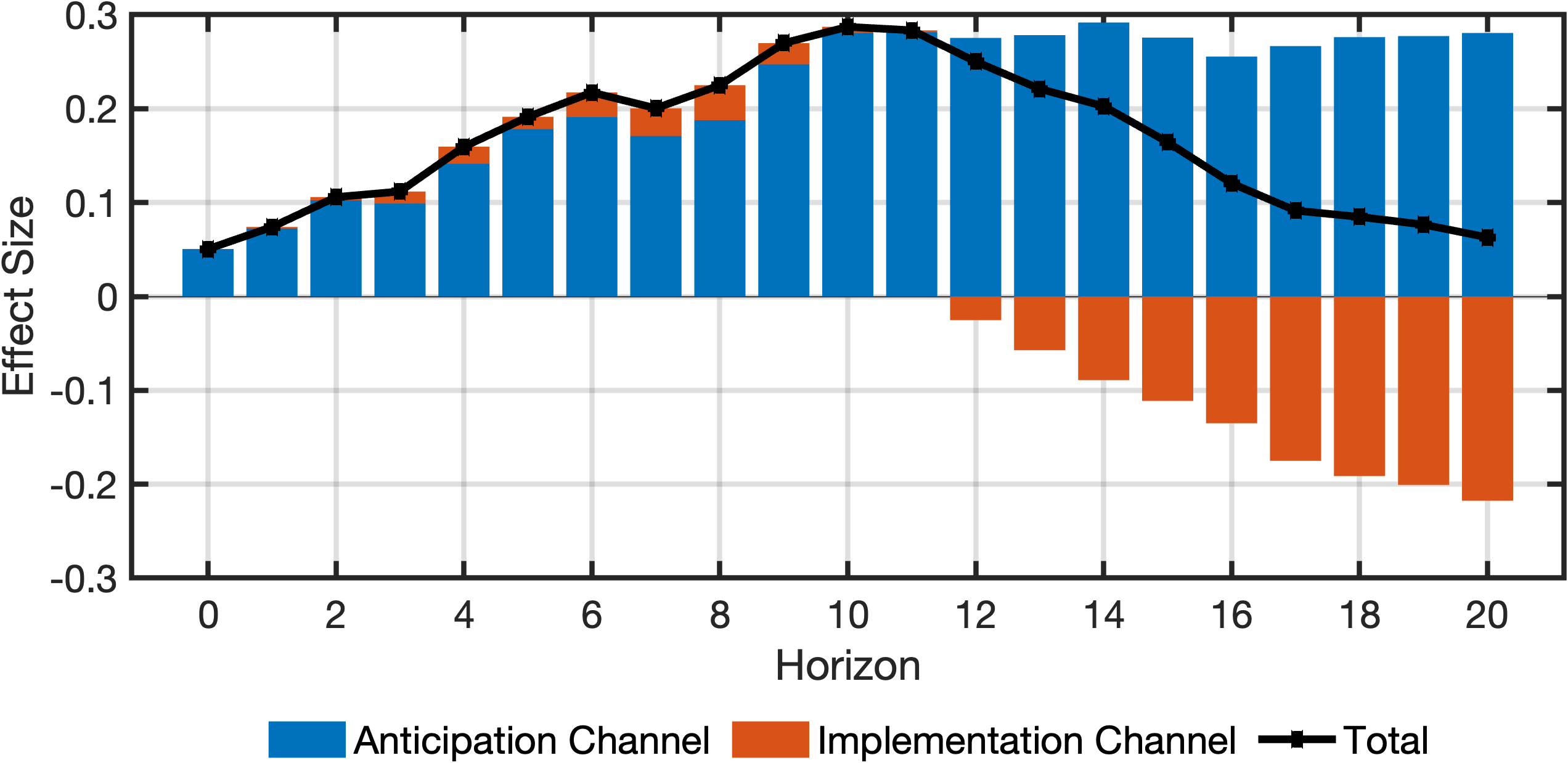
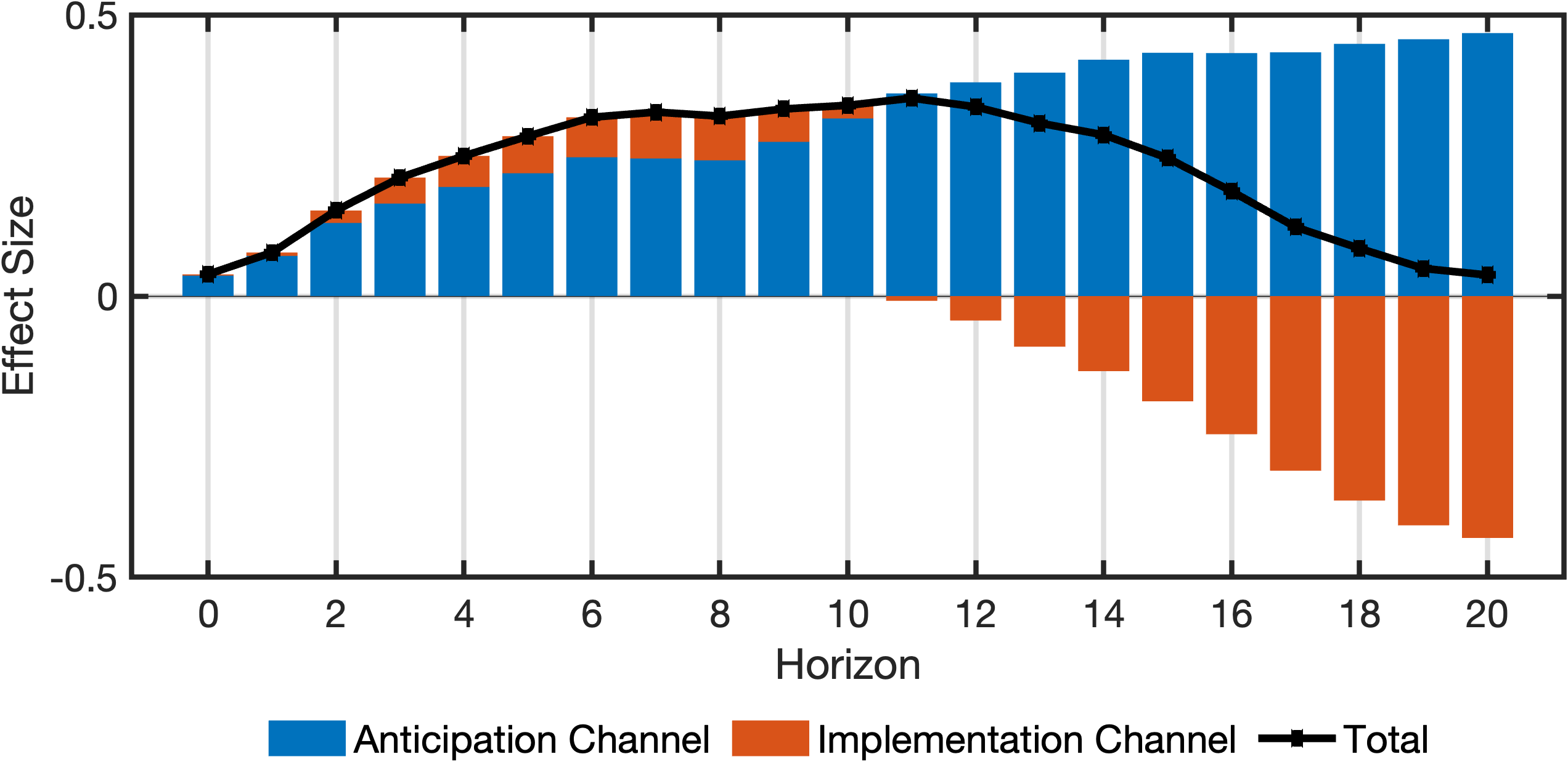
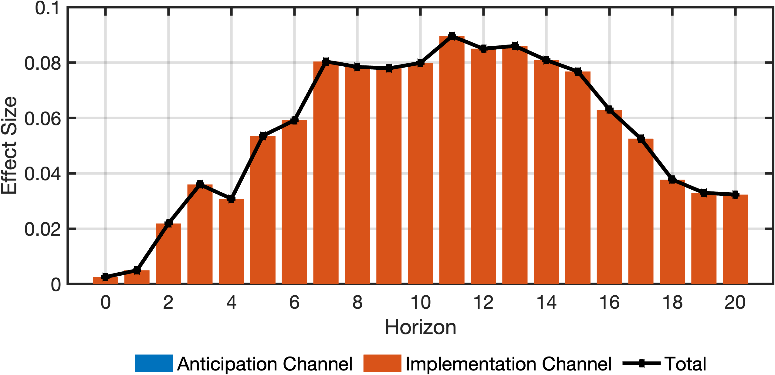
cellChannelEffects = {anticipationEffects, implementationEffects};Figures Figure 1 (a) to Figure 1 (c) illustrate decompositions for output, total government spending, and government defense spending, respectively. These can be obtained using:
% output
fig = plotDecomposition(4, irfs(:, 1, :), cellChannelEffects, channelNames)
% Total government spending
fig = plotDecomposition(3, irfs(:, 1, :), cellChannelEffects, channelNames)% Government defense spending
fig = plotDecomposition(2, irfs(:, 1, :), cellChannelEffects, channelNames)