R <- 100000 # number of Monte Carlo repetitions
n <- 10 # number of uniform random variables
Y <- rep(0, R) # vector to store the maxima
for (r in 1:R) {
  X <- runif(n) # draw X_1 to X_n from uniform distribution
  Y[r] <- max(X) # compute maximum of X_1 to X_n for the rth repetition
}10 Monte Carlo simulations
Sometimes we are confronted with problems that are difficult or even impossible to solve with standard mathematical or statistical methods. Often we can solve such problems by using a Monte Carlo approach. The basic idea is that instead of evaluating a complicated integral involving some probability density function we sample from the corresponding distribution many times and take the average of
To illustrate the approach suppose that \(X_1,\ldots,X_n\) are independent and uniformly distributed on the interval \([0,1]\) and that we are interested in the distribution of the maximum, \[ Y=\max\{X_1,\ldots,X_n\}. \] Although in this case we can derive the CDF and the PDF of \(Y\) theoretically (and we will do so later in the course) we can use a Monte Carlo simulation to approximate the distribution of \(Y\) and any derived quantities of interest such as the mean or the variance.
The above code uses a for loop to realize the Monte Carlo repetitions. Although since version 3.4 R has a just-in-time compilation that improves runtime performance of loops considerably, an alternative implementation using apply and its variants still can yield slightly faster code.
R <- 100000
n <- 10
X <- runif(n * R)
dim(X) <- c(n, R)
Y <- apply(X, 2, max)
In this implementation all necessary memory is allocated at once and thus leads to a (slight) improvement in running time. The generated random values are grouped into a matrix where each column contains \(X_1,\ldots,X_n\) for a single repetition. The apply command is used to compute the maximum \(Y\) for each repetition (i.e. column).
Another alternative implementation makes use of the replicate command. The code is self-documenting but leads to slightly higher running times.
R <- 100000
n <- 10
Y <- replicate(R, max(runif(n)))
With each approrach we obtain a vector Y of length R which contains repeated realizations of the random variable \(Y\). With these values we can approximate any probability of interest, such as the probability that \(Y>\tfrac{1}{2}\), by the corresponding empirical proportion:
p <- mean(Y > 0.9)
p
[1] 0.65105Similarly, we can approximate the mean of \(Y\) by the average of the simulated outcomes in Y, and the PDF of \(Y\) can be visualized by a histogram:
# plot histogram and print mean and variance
hist(Y, breaks = seq(0, 1, length = 101), freq = FALSE)
text(0, 9 * max(Y), paste("E(Y)=", format(mean(Y), digit = 4), sep = ""), adj = c(0, 0))
text(0, 8 * max(Y), paste("var(Y)=", format(var(Y), digit = 4), sep = ""), adj = c(0, 0))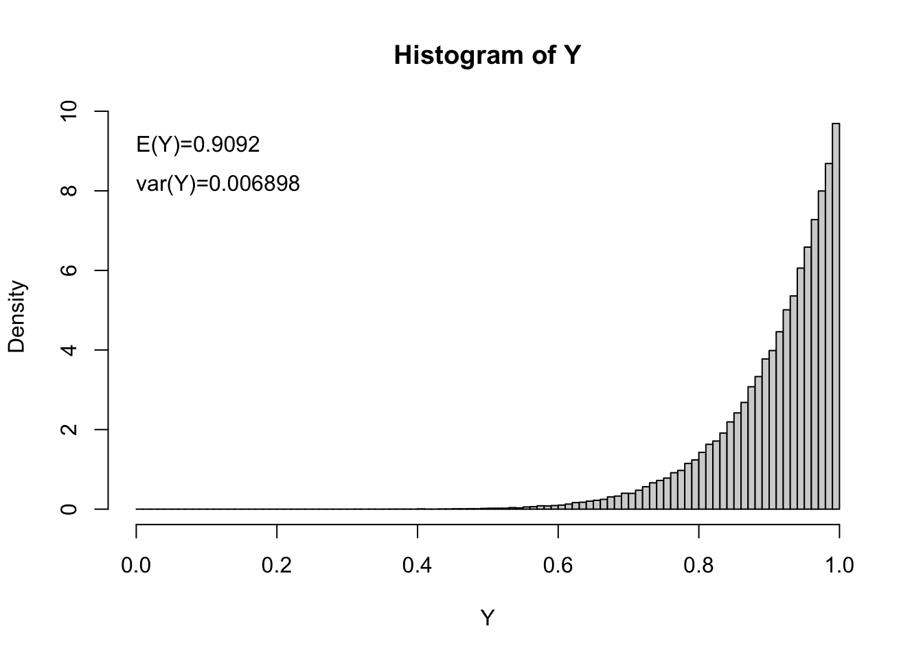
As a second, slightly more advanced example let us assume that we hold a call option on a stock. The option pays at some fixed future time \(T\) the amount by which the price \(S_T\) of one share in the underlying stock exceeds a fixed price \(K\) (the so-called strike price of the call option). In order to value our investment we might be interested in
- the expected pay-off of the call option: \(\mathbb{E}\big(\max(S_T-K,0)\big)\);
- the probability of the call option expiring worthless: \(\mathbb{P}(S_T<K)\);
- the probability of the call option exceeding some value \(c^*\): \(\mathbb{P}(C_T>c^*)=\mathbb{P}(S_T>K+c^*)\);
- the complete distribution of the pay-off of the option.
For simplicity we assume that the yearly log-returns of the stock are normally distributed with mean \(\mu=0.1\) and standard deviation \(\sigma=0.2\). Furthermore, we assume that the option expires in half a year, that the current value of one share of the stock is \(S_0=100\) and that \(c^*=120\) (both in €).
N <- 100000
mu <- 0.1
sigma <- 0.2
T <- 0.5
start_value <- 100
Strike <- 110
threshold <- 120
Z <- rnorm(N)
final_value <- start_value * exp(mu * T + sigma * sqrt(T) * Z)
call_payoff <- ifelse(final_value > Strike, final_value - Strike, 0)
ave_payoff <- mean(call_payoff)
p_zeropayoff <- mean(call_payoff <= 0)
p_threshold <- mean(call_payoff > threshold)
hist(call_payoff[call_payoff > 0], breaks = 100, freq = FALSE, main = "Histogram of positive payoffs", xlab = "payoff")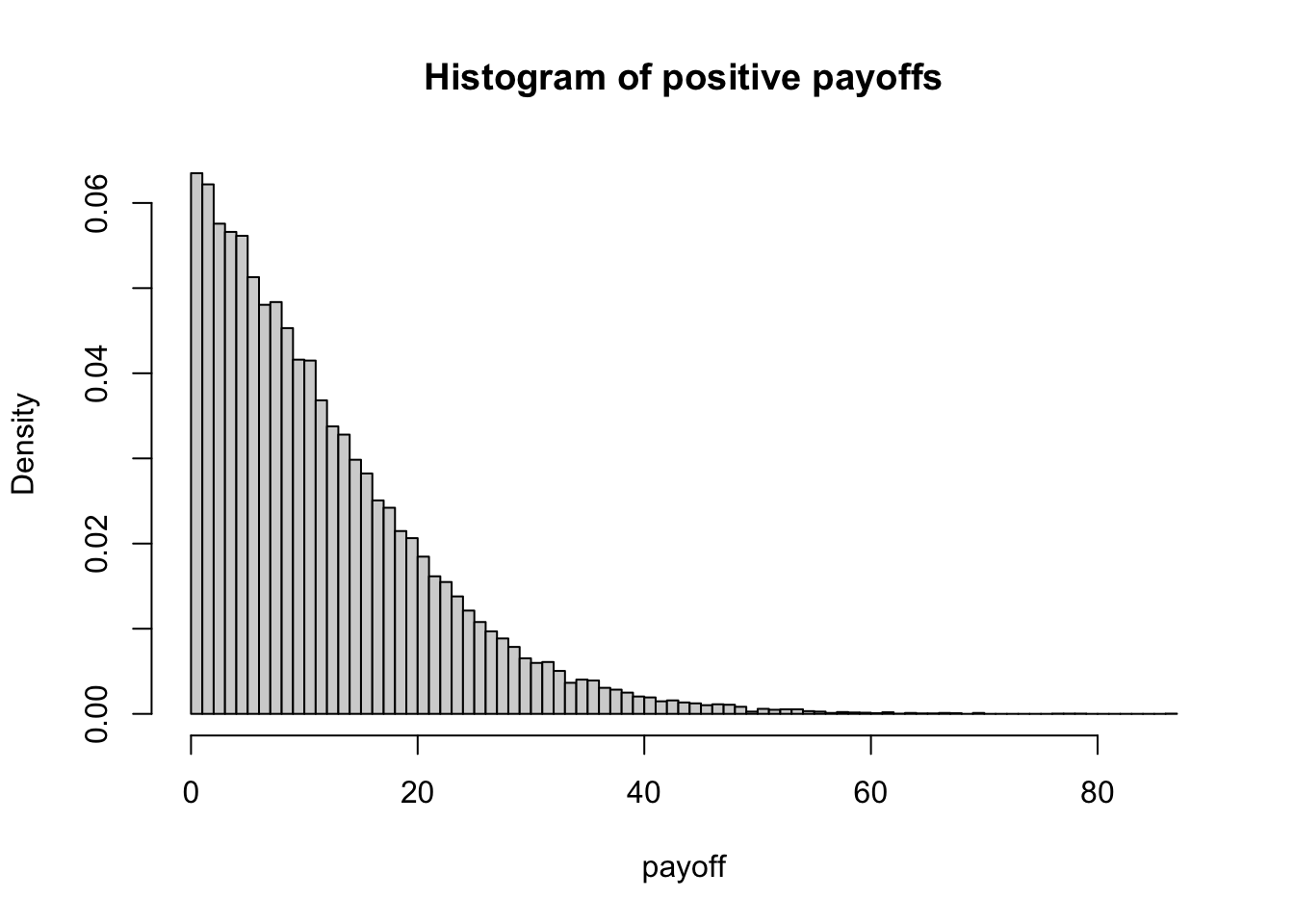
While the above probabilities and means can be derived exactly by analytic manipulations, computations become infeasible if we replace the normal distribution of the log-returns by a t distribution with \(v\) degrees of freedom. For small \(v\) the \(t\) distribution tends to have more extreme values than the normal distribution and thus might be more realistic choice for the distribution of the log-returns. The code for the Monte Carlo simulation, on the other hand, can be straightforwardly adapted to this change of the underlying distribution by replacing the line Z=rnorm(N) by Z=rt(N,df=v) and defining v at the beginning of the code (e.g. v=5 assures that the log-returns still have finite kurtosis.)
10.1 A case study
Imagine you are working for a large pension fund and you have figured out that the monthly return on your portfolio is approximately normally distributed with mean \(\mu\) and standard deviation \(\sigma\). Because you work for a pension fund, you have monthly expenses in the form of pension payments to clients. You are afraid of not being able to make these payments and thus start looking for ways to insure that you can make the payments over the next \(T\) years. A bank you have worked with before offers you a financial product. Every month that your portfolio does not return enough money to pay for the monthly payment of \(x\) euros, they will match the difference, therefore allowing you to still pay \(x\) euros. In return, they request to get \(y\) cents on any euro you make above the \(x\) euros in each month. Additionally, they request a one-off payment of \(z\) euros. For now we abstract away from all the other problems and instead your task as the econometrician in the company is to figure out how much you are expected to pay the bank and how much they are expected to pay you over the next \(T\) years.
simulate_payment <- function(start_value, mu, sigma, T, x, y, z) {
  num_months <- T * 12
1  returns <- rnorm(num_months, mu, sigma)
2  money_received <- 0
  money_paid <- z
  portfolio_value <- rep(NA, num_months)
  portfolio_value[1] <- start_value
3  for (t in 2:(num_months + 1)) {
    gain <- portfolio_value[t - 1] * returns[t - 1]
    if (gain >= x) {
      left_over_gain <- gain - x
      to_pay <- y / 100 * left_over_gain
      left_over_gain <- left_over_gain - to_pay
      portfolio_value[t] <- portfolio_value[t - 1] + left_over_gain
      money_paid <- money_paid + to_pay
    } else {
      money_received <- money_received + min(c(x - gain, x))
      portfolio_value[t] <- portfolio_value[t - 1] + min(c(gain, 0))
    }
  }
  out <- list(
    portfolio_value = portfolio_value[num_months + 1],
    money_paid = money_paid,
    money_received = money_received
  )
  return(out)
}- 1
- draw the random returns from the normal distribution
- 2
- create variables to store simulation results
- 3
-
loop over each period. We start at period
t=2because time one is the starting time
start_value <- 10000
mu <- 0.01
sigma <- 0.06
T <- 10
x <- 70
y <- 10
z <- 100
results <- simulate_payment(start_value, mu, sigma, T, x, y, z)
rbind(results)
portfolio_value money_paid money_received
results 16634.16 3247.452 4090.59 The following code generates the Monte Carlo repetitions to compute the expected values.
expected_payments <- function(n, start_value, mu, sigma, T, x, y, z, seed) {
  if (!missing(seed)) set.seed(seed) # set seed if provided
  f <- function(i) unlist(simulate_payment(start_value, mu, sigma, T, x, y, z))
  outputs <- sapply(1:n, f, simplify = TRUE)
  mean_outputs <- apply(outputs, 1, mean)
  return(mean_outputs)
}
# example values
mu <- 0.01
sigma <- 0.06
T <- 10
x <- 70
y <- 10
z <- 50
start_value <- 10000
outputs <- expected_payments(10000, start_value, mu, sigma, T, x, y, z)
outputs
portfolio_value money_paid money_received
16935.694 4160.511 3826.225 Finally we compute the expected gain or loss from the contract for a range of monthly costs.
value_contract <- function(n, xs, start_value, mu, sigma, T, y, z) {
  f <- function(x) c(expected_payments(n, start_value, mu, sigma, T, x, y, z), x = x)
  exp_pay <- sapply(xs, f)
  exp_value <- exp_pay["money_received", ] - exp_pay["money_paid", ]
  output <- cbind(exp_value, exp_pay["x", ])
  colnames(output) <- c("Expected Value", "X")
  return(output)
}

# compute expected gain/loss for range of monthly costs

mu <- 0.01
sigma <- 0.06
T <- 10
y <- 10
z <- 50
start_value <- 10000
value <- value_contract(10000, seq(60, 90, 2), start_value = start_value, T = T, y = y, z = z, mu = mu, sigma = sigma)
# plot a curve showing the expected gain/loss for chosen range of monthly costs

par(mar = c(2.5, 2.5, 0.5, 0.5), mgp = c(1.4, 0.2, 0), cex = 0.7, bty = "l", las = 1, lwd = 0.5, tck = 0.01)
plot(value[, "X"],
  value[, "Expected Value"],
  type = "l",
  xlab = "Monthly cost x [K€]",
  ylab = "Expected payoff of contract [K€]"
)
abline(h = 0, col = "black", lty = 3)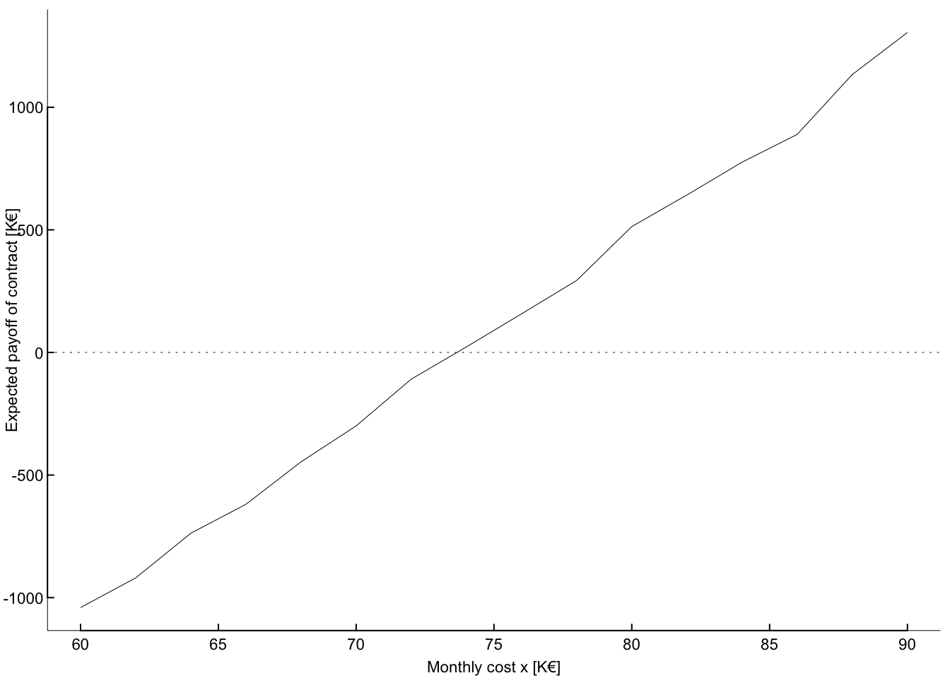
Since the value of the portfolio at time \(t\) depends on the value at time \(t-1\), the simulation of the portfolio values over time cannot be vectorized. However, instead of looping for each Monte Carlo repetition separately, we can make use of vectorized computations by stacking all repetitions into one vector. In order to execute conditional statements elementwise we note that the price of the portfolio at time \(t\) can be written as \[
\Pi_t=(1-y)G_t\,1_{\{G_t>x\}}+G_t\,1_{\{G_t<0\}}.
\] where \(G_t=\Pi_{t-1}\,r_t\) is the gain or loss of the portfolio and \(r_t\) is the return of the portfolio. The indicator functions cen be implemented by using the ifelse function.
simulate_payments <- function(n, start_value, mu, sigma, T, x, y, z) {
  num_months <- T * 12
  returns <- rnorm(num_months * n, mu, sigma)
  dim(returns) <- c(num_months, n)
  money_received <- rep(0, n)
  money_paid <- rep(z, n)
  portfolio_value <- rep(start_value, n)
  for (t in 1:num_months) {
    gain <- portfolio_value * returns[t, ]
    gtx <- ifelse(gain > x, 1, 0)
    gtzero <- ifelse(gain > 0, 1, 0)
    left_over_gain <- gtx * (gain - x)
    to_pay <- (y / 100) * left_over_gain
    to_receive <- (1 - gtx) * (x - gtzero * gain)
    money_paid <- money_paid + to_pay
    money_received <- money_received + to_receive
    portfolio_value <- portfolio_value + left_over_gain - to_pay + (1 - gtzero) * gain
  }
  out <- list(
    portfolio_value = portfolio_value,
    money_paid = money_paid,
    money_received = money_received
  )
  return(out)
}
The rest of the code is similar to that of the first approach.
mu <- 0.01
sigma <- 0.06
T <- 10
x <- 70
y <- 10
z <- 50
start_value <- 10000
S <- rep(0, 12 * T + 1)
result <- simulate_payments(1, start_value, mu, sigma, T, x, y, z)
output <- lapply(result, mean)
output
$portfolio_value
[1] 13891.06
$money_paid
[1] 3245.333
$money_received
[1] 3655.362value_contract <- function(n, xs, start_value, mu, sigma, T, y, z) {
L <- length(xs)
output <- matrix(NA, L, 2)
for (i in 1:L) {
result <- simulate_payments(n, start_value, mu, sigma, T, xs[i], y, z)
output[i, ] <- c(mean(result$money_received - result$money_paid), xs[i])
}
colnames(output) <- c("Expected Value", "X")
return(output)
}
# initialize parameter values
mu <- 0.01
sigma <- 0.06
T <- 10
x <- 70
y <- 10
z <- 50
start_value <- 10000
# range of values for which the expected gain/loss is computed
xs <- seq(60, 90, 2)
value <- value_contract(10000, xs, start_value, mu, sigma, T, y = y, z = z)
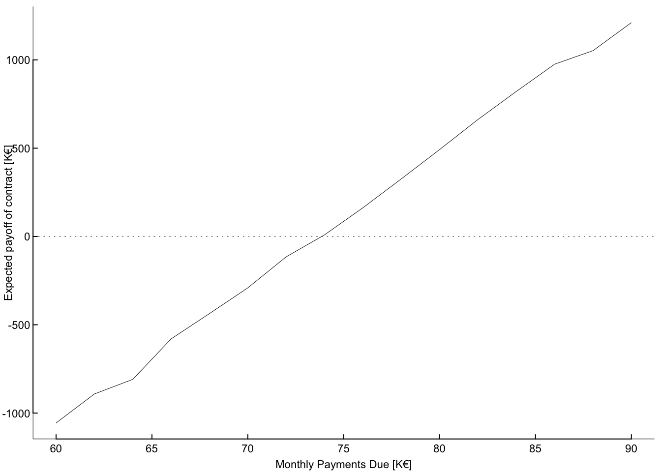
par(mar = c(2.5, 2.5, 0.5, 0.5), mgp = c(1.4, 0.2, 0), cex = 0.7, bty = "l", las = 1, lwd = 0.5, tck = 0.01)
plot(value[, "X"],
value[, "Expected Value"],
type = "l",
xlab = "Monthly Payments Due [K€]",
ylab = "Expected payoff of contract [K€]"
)
abline(h = 0, col = "black", lty = 3)