runif(1)[1] 0.9903114Random numbers and random variables play an important role in probability theory. So do distributions of these random variables. While you will later learn what random variables and distributions are, we will here introduce the basics of them in R.
Imagine rolling two dice and summing the outcome of the two. The value you obtain is a random number and if we assign it a meaning, it is a random variable. Why is it random? Simply because the outcome of each die was random. If you repeat the experiment you are likely to get new values. Now, computers cannot role die for us and thus they cannot generate truly random numbers. However, what they are incredible good at is to simulate values that are as good as random for any practical purposes. How they do this is beyond the scope of these notes, but feel free to look it up online.
An example of a random number is a value between zero and one with each value being equally likely to appear. We call this a uniform distribution on the interval \((0,1)\) (denoted as \(\text{Unif}(0,1)\)) and we can obtain a value from this distribution by running
runif(1)[1] 0.9903114Each time you run the above line you will get a different value and you will not be able to predict the next value no matter how many of the previous values you saved and what algorithm you are using. This is why we call these numbers random in any practical sense.
The uniform distribution can also be extended to larger and smaller values. For example, we might want to obtain a random value between -10 and 10 with all values being equally likely. This is an example of a \(\text{Unif}(-10, 10)\) distribution, and similar to above, we can obtain a draw from this distribution by simply providing the min and max values of the uniform distribution.
runif(1, min = -10, max = 10)[1] -0.8965356What if we need more than one value? R makes this rather simple and usually the first argument to any distribution is the number of draws you want from that distribution. So instead of choosing 1 as in the code above, we could also choose 10 to obtain ten values of the same distribution. Since all values are equally likely, there is a zero probability that any of the ten values will be the same. Do not worry if this does not yet make sense. At the end of the course you will understand why. And if you do not trust us, feel free to sample one million values and check if any of them are the same.
runif(10, min = -10, max = 10) [1] -5.3106017 2.5112541 -6.8677151 3.5847242 -0.8365961 -5.7187392
[7] -6.0189922 -6.7606133 9.7952046 9.9240900The ability to sample multiple values from the same distribution also allows us to obtain a random matrix for which each element is drawn independently from the same distribution. Independence means that knowing the value of one entry in the matrix will tell you nothing about what the other values will be. We will formalise this definition later on. To sample a random matrix with each element coming from the same distribution, we simply sample enough draws from the distribution and reshape it into a matrix.
matrix(runif(10*5, min = -10, max = 10), nrow = 10) [,1] [,2] [,3] [,4] [,5]
[1,] -3.5713130 -0.37518264 0.9699592 4.254513 -4.1082568
[2,] 0.4611284 1.31943360 -2.4485040 -8.413718 -6.7193400
[3,] 9.5447636 -0.03986039 5.6719692 -5.723925 2.3496357
[4,] -1.2187543 0.52472583 -0.2942319 7.550407 0.3444718
[5,] 3.5018049 3.00888106 -6.7831378 2.019172 2.6677826
[6,] 2.4875952 0.35353755 6.2483188 4.838260 -4.7636075
[7,] -2.6427121 5.32370195 -6.6053319 3.902200 -8.6431233
[8,] 0.8316657 -8.29043168 -1.8350054 -2.570487 9.0103183
[9,] -0.1884462 7.94606084 2.0239705 9.414560 -2.5768445
[10,] -0.9626703 8.80552080 -0.3061083 -2.292461 2.3814311What if we wanted to draw from another distribution? Many commonly used distributions exist and you will encounter many of them during this course. R implements most of them, with Table 9.1 providing an overview of the functions used for each distribution. Thus far we have only used the r* function and we will show the use of a d* functions below. We will encounter the other functions throughout the remainder of this course.
| Distribution | PDF/PMF | CDF | Quantile Function | Random Variate |
|---|---|---|---|---|
| Beta | dbeta |
pbeta |
qbeta |
rbeta |
| Binomial | dbinom |
pbinom |
qbinom |
rbinom |
| Cauchy | dcauchy |
pcauchy |
qcauchy |
rcauchy |
| Chi-Squared | dchisq |
pchisq |
qchisq |
rchisq |
| Exponential | dexp |
pexp |
qexp |
rexp |
| F | df |
pf |
qf |
rf |
| Gamma | dgamma |
pgamma |
qgamma |
rgamma |
| Geometric | dgeom |
pgeom |
qgeom |
rgeom |
| Hypergeometric | dhyper |
phyper |
qhyper |
rhyper |
| log-Normal | dlnorm |
plnorm |
qlnorm |
rlnorm |
| Multinomial | dmultinom |
pmultinom |
qmultinom |
rmultinom |
| Negative Binomial | dnbinom |
pnbinom |
qnbinom |
rnbinom |
| Normal | dnorm |
pnorm |
qnorm |
rnorm |
| Poisson | dpois |
ppois |
qpois |
rpois |
| Student’s t | dt |
pt |
qt |
rt |
| Uniform (Cont.) | dunif |
punif |
qunif |
runif |
| Weibull | dweibull |
pweibull |
qweibull |
rweibull |
According to Table 9.1, to draw from the normal/Gaussian distribution, we should use rnorm. The normal distribution does not have the same arguments as the uniform distribution though. Thus, even though we can just call rnorm(1), we will not get a value between 0 and 1 as in the runif(1) case. Instead, the value could theoretically be anything, with the value most likely being somewhere between -3 and 3.
rnorm(1)[1] -0.55308rnorm(1, mean = 10, sd = 4)[1] 4.49151rnorm(10, mean = 10, sd = 4) [1] 3.732157 10.210965 10.672211 14.381870 8.046368 17.521572 8.480063
[8] 10.082053 14.502437 13.131405matrix(rnorm(10*5, mean = 10, sd = 4), nrow = 10) [,1] [,2] [,3] [,4] [,5]
[1,] 4.335116 11.5046995 9.697173 8.651911 7.605066
[2,] 5.819922 10.1137624 2.982633 10.154907 7.705984
[3,] 7.276580 0.6449421 13.223495 9.650778 6.202145
[4,] 7.514405 11.6379204 12.023304 4.788214 8.207524
[5,] 15.695662 9.2776879 11.293142 9.858663 5.455217
[6,] 13.520527 9.6431797 16.478934 11.603003 9.202656
[7,] 9.824702 -1.8222605 3.261466 11.507411 11.581257
[8,] 9.012902 11.4024169 11.149051 2.593784 9.641504
[9,] 6.904652 11.6440788 13.801578 6.093255 18.953835
[10,] 7.085981 8.9264889 6.969944 12.321976 6.293552While the uniform distribution is parameterised by the minimum and maximum values, the normal distribution is parameterised by the mean and standard deviation. Both are already used above to obtain different random values from the normal distribution, but if you want to know more about this parameterisation and the normal distribution, you can always ask the help.
?rnormAnother distribution you will encounter in the course is the Beta distribution. In contrast to the normal and the uniform distribution, there exist no universally agreed upon default parameters for the Beta distribution, and thus rbeta(1) does not work. Instead, every time you want to draw a value from the Beta distribution, you need to specify its shape, which you can do by specifying two more arguments after the number of draws. Also check out ?rbeta.
rbeta(1, 1, 1)[1] 0.4284701How does this Beta distribution look like? And how do the uniform and normal distributions look like? We can use the skills we developed so far to figure this out. First, we can draw a large number of draws from the Beta distribution. We can then plot the density histogram of these draws to get an idea of how the distribution looks like.
draws_beta <- rbeta(1000, 1, 1)
hist(draws_beta, breaks = 50, freq = FALSE, xlab = "x", main = "")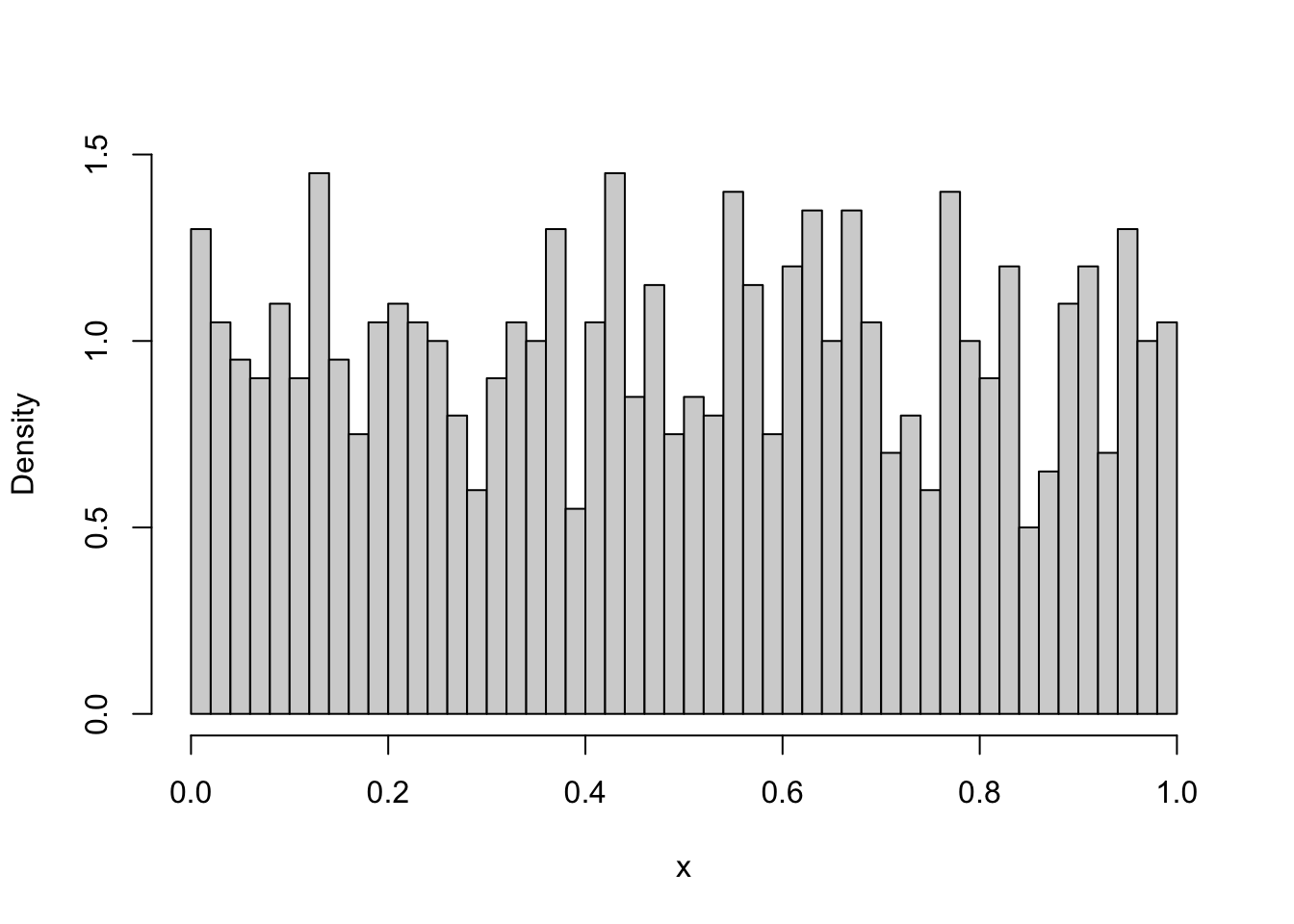
The obtained histogram depends on the random draws and thus will give you only a (random) approximation to the distribution. Alternatively, we can also plot the theoretical density. The dbeta function provides the density of the Beta function at any point. Thus, we can simply define the x range over which we want to plot the Beta density, then create a sequence of x points within that range and calculate the density at each of these points. This can then be plotted to get an even better understanding of how the theoretical density looks like.
x <- seq(0, 1, 0.01)
density_beta <- dbeta(x, 1, 1)
plot(x, density_beta, type = "l", ylab = "Density")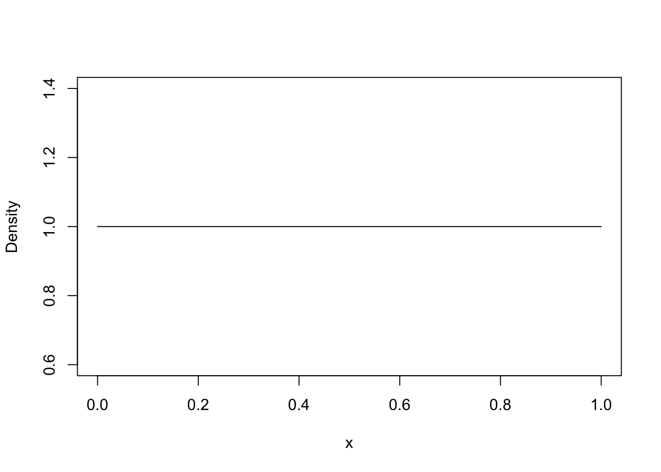
With 10000 draws, the empirical density was quite close to the theoretical density. We could compare these two more easily if we plot them in the same plot. Additionally, we might ask just how many of these draws we need for a reasonably precise answer, and how the Beta distribution looks like for various parameter values. Thus, we would like to do the same thing multiple times, each time only changing a small part of the code. By now, this should ring a bell: A function is needed! Below we implement a function that allows us to compare the empirical and theoretical density for various parameterisations and number of draws.
#' Compares the empirical and theoretical density of a Beta distribution
#'
#' @param n Number of draws to take for the empirical density
#' @param shape1 Shape parameter of Beta. See ?rbeta.
#' @param shape2 Shape parameter of Beta. See ?rbeta.
#' @param step_size Controls the details of the theoretical density plot.
#' The smaller this value, the more detailed the plot. Default value is 0.01.
#' @return Returns a plot.
#' @examples
#' plot_beta_density(10000, 1, 1)
#' plot_beta_density(10000, 1, 5, step_size=1e-4)
plot_beta_density <- function(n, shape1, shape2, step_size=0.01){
  draws_beta <- rbeta(n, shape1, shape2)
  min_x <- min(draws_beta)
  max_x <- max(draws_beta)
  x <- seq(min_x, max_x, step_size)
  density_beta <- dbeta(x, shape1, shape2)
  hist(draws_beta,
       breaks = 50,
       freq = FALSE,
       xlab = "x",
       ylab = "Density",
       main = sprintf("Beta(%.2f, %.2f)", shape1, shape2)
       )
  lines(x, density_beta, col="black", lwd = 2)
}
Even better than above, we can see that the empirical density is very close to the theoretical density if we use 10000 draws.
plot_beta_density(10000, 1, 1)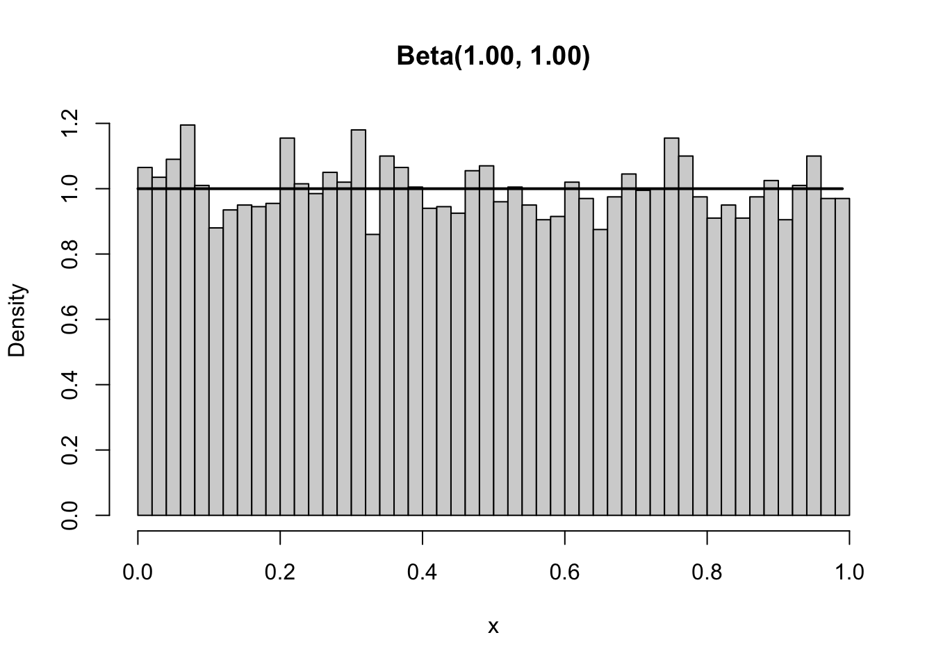
However, using the function we can easily check if this is also the case if we use different parameters for the Beta and thus obtain a different shape. As shown below, changing the second shape to 4 changes the Beta distribution from a horizontal line between 0 and 1 to a a downward sloping line with the majority of the density being close to zero. The approximation of the empirical density is still good.
plot_beta_density(10000, 1, 4)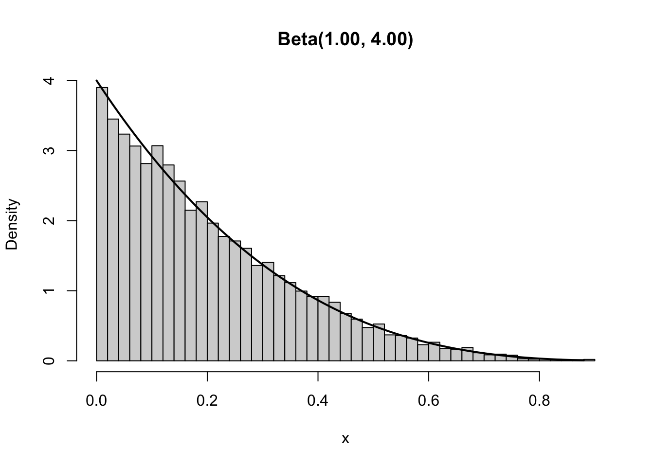
The empiricial density becomes a worse approximation if we draw fewer values from the Beta distribution. We can easily show this by using our plot_beta_density function and simply choosing fewer values to draw from the distribution. Below we show what happens if we only draw 100 values from the distribution. Clearly, the empirical distribution is far from the theoretical.
plot_beta_density(100, 1, 4)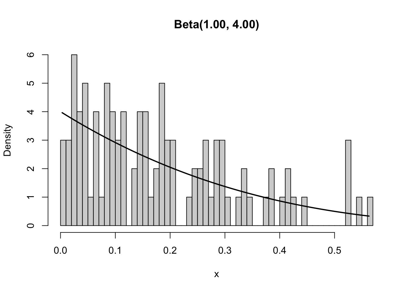
Since distributions play an important role in probability theory and statistics, it is no surprise that many great resources exist. One of our favourite resources is the Distribution Zoo which depicts the shapes of various distributions, provides R implementation details, and gives some details on when to use which distribution.
We already pointed out above that if we rerun a line of code that draws a random number, we obtain a new value. A consequence of this is that every time we rerun the plot_beta_density function we obtain a slightly different plot. This can cause problems especially when the functions are more complex. For example, if we had only given you the graph and asked you to replicate the graph using your knowledge, how would you know whether your function is correct? The difference in your and our plot might be due to randomness or it might be due to a mistake in your code. This is a replicability problem.
plot_beta_density(100, 1, 4)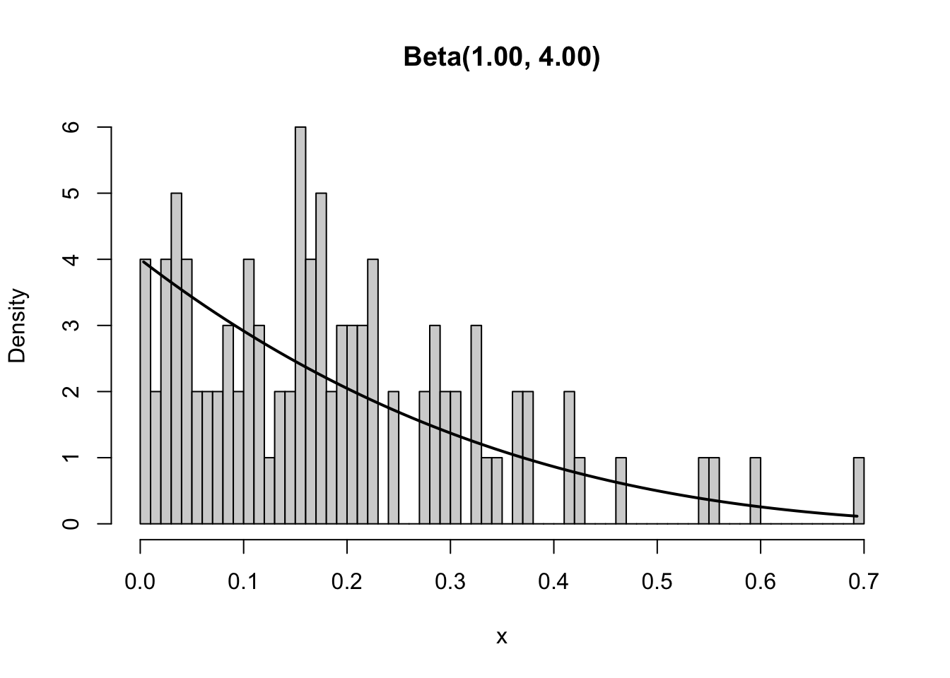
Replicability is an important problem in science. Only results that can be replicated should be trusted. Unfortunately, many scientific results are difficult to replicate or are just never replicated for other reasons. Nonetheless, we should always aim at making our work as replicable as possible. This is not just for others, but also for ourselves. Sometimes we need to obtain the same graph again because we might have to change the title. If the function provides a new graph each time, it becomes difficult to convince anyone that we actually used the same graph as before. Thus, we have to make our code replicable. Clean code is a first step towards that, but if we use randomness, we also need to use a seed.
A seed assures that each time we run the code, we will obtain exactly the same results. The emphasis is on run the same code. We only obtain the same result if we run everything after the line at which we set the seed. To set a seed, we use set.seed and provide any integer to it. A good practice is to use a large integer, but even set.seed(1) is better than not setting any seed.
set.seed(6150533)
rgamma(1, 1)
[1] 1.583487Now that the seed is set, we can run the same code as above and obtain the exact same result as before.
set.seed(6150533)
rgamma(1, 1)
[1] 1.583487The downside of using a seed is that no matter how many times you run the above code you always will get the same value - quite the opposite of what you should expect of a random number! So while exploring some random quantity you do not want to reset the seed again and again to the same value. However, when starting to collect your results you need to set the seed (e.g. at the beginning of your submitted code) in order to make your results reproducible.
R itself initialises its random number generators by use of the current time and some process ID. You can make use of this quite arbitrary initialisation by choosing the seed itself at random:
sample(100000000,1)[1] 65192504set.seed(45489699)